Inflation did not vanish after a couple of noisy prints. It returned as a regime that tests how we measure risk, price growth, and size the portfolio. Factor models that ignore that regime change miss where returns and risks actually come from.
What “inflation‑adjusted” factor models are
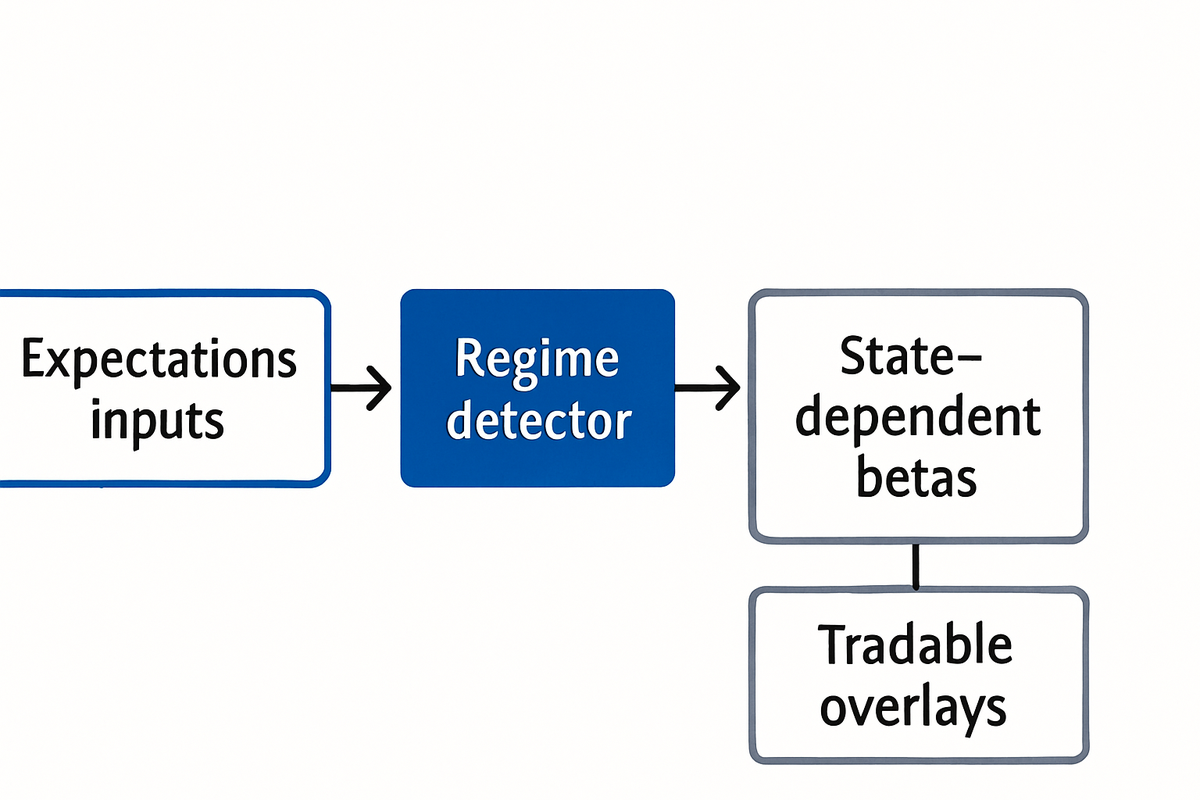
An inflation‑adjusted factor model is a standard multifactor framework that makes its moving parts depend on inflation signals. The signals include breakeven rates, survey expectations, real rates, and commodity proxies. The framework also allows for discrete regimes that can flip the behaviour of betas and premia.
It is not the same as bolting on a single “inflation factor.” Adding one proxy and hoping it absorbs the shock is a weak fix. A richer design allows factor returns, betas, and prices of risk to vary with observable inflation states.
Institutional practice points in the same direction. A systematic approach that treats inflation and real rates as explicit macro drivers, and that implements tilts with TIPS and commodities, has been laid out by BlackRock Systematic’s Market Advantage framework.
There is also a behavioural piece. Inflation expectations shape the path that inflation takes, which then shapes the response of policy and markets. That loop is central in BIS Working Paper No 1060 by Ricardo Reis and it is why expectations data must enter the model as a state variable.
Why now: the 2021–22 stress test
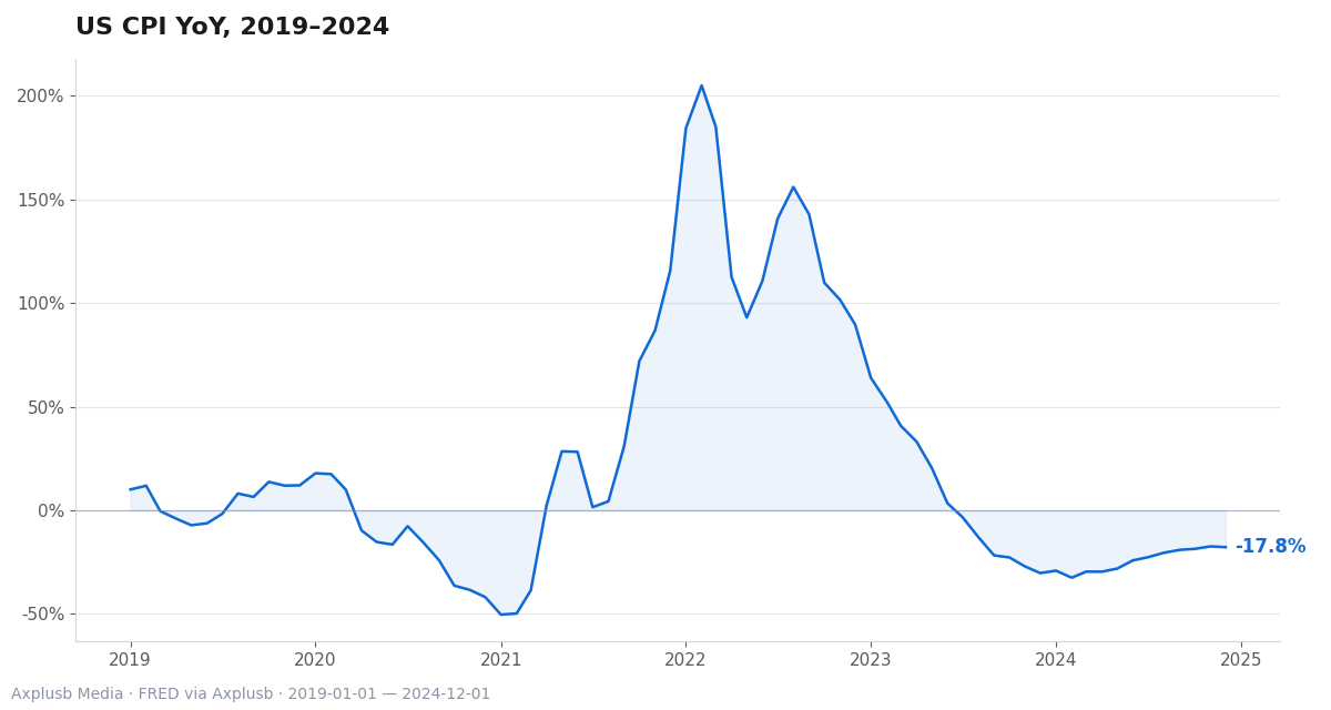
The 2021–22 burst exposed a gap between models that assume stable betas and the world we actually live in. The shock lasted longer because expectations moved and policy adapted in real time. Static models with fixed parameters did not recognize that shift until it was too late.
The episode also surfaced a practical distinction. When inflation is driven by supply shocks, stress in the system responds differently to policy than when demand is strong. A model that cannot separate those states will mix signals and misprice risk.
These dynamics did not only affect macro series. They filtered into factor behaviour, sector leadership, and cross‑asset spreads. If a model did not respond to regime clues, it lagged in both risk control and tilt selection.
Finally, the episode invited a simple test. Did your factor model adjust exposures when breakevens and surveys moved sharply, or did it bake in priors from the disinflation era?
The core modelling gaps to close
Most gaps are practical and fixable. Four stand out across teams and tools.
First, regime detection. We need a method to detect discrete shifts in inflation dynamics, rather than assuming a slow drift. Those shifts can flip the sign of a beta and change how shocks propagate.
Second, expectations as state variables. Breakevens, survey paths, and real‑rate levels should drive time‑varying betas and premia. This is the difference between reacting to realized CPI and conditioning on investor beliefs.
Third, a bond factor that respects real versus nominal. A term‑premium estimate helps separate duration risk from expected paths. The New York Fed’s Adrian–Crump–Moench approach is a ready method and a long history for this job.
Fourth, time‑varying, state‑dependent betas and prices of risk. The econometric frame should let factor loadings and premia move with inflation states. Without it, the model treats a 2014 regime like a 2022 regime.
| Gap to Close | Practical Ingredient |
|---|---|
| Regime detection | Markov/threshold switching on factor loadings |
| Expectations as states | Breakevens, survey paths, real rates as regressors |
| Bond factor realism | Term-premium estimate, real vs nominal split |
| Time-variation in risk | State-dependent betas and prices of risk |
A consistent message from long horizon research is to respect diversification while adding these pieces. Multifactor portfolios remain robust on average, yet factor sensitivities vary across growth and inflation regimes, as documented in AQR’s Quant Special Issue on Fact and Fiction in factor investing.
Econometric toolbox: estimating time variation and regimes
You do not need exotic machinery to start. A regression‑based dynamic asset pricing setup can allow prices of risk to move with state variables. Factor betas can then be estimated in rolling windows or in a two‑step system.
The next layer is regime switching. An expectation‑maximization algorithm with a Markov or threshold switch can spot discrete changes in factor loadings. This method captures jumps that a simple linear trend would miss.
Bring those two pieces together to get a workable backbone. Time‑varying prices of risk handle the drift that comes with changing expectations. Regime switches handle the breaks that come with policy or supply shocks.
Estimation is not the only challenge. Inference under switching must guard against overfitting and spuriously detected regimes, which is common when the model is high dimensional.
Time‑varying betas in practice
Start simple and observable. Let betas vary with one or two inflation signals, such as 5‑year breakevens and a survey measure. Estimate betas with a lag to avoid look‑ahead, and monitor stability across windows.
Then add cross‑checks. Compare the implied exposures from the model with exposures seen in traded products. Large gaps can reveal instability in the state mapping.
Regime switching without drama
Use a small number of regimes. Two or three states are often enough for inflation dynamics. More states make interpretation harder and raise the odds of false detection.
Impose economic priors where possible. For example, require that a “high inflation” regime lines up with thresholds in the signal, or with sustained moves in breakevens. Priors can stabilize estimation when the data are noisy.
Which signals and instruments to use in practice
The signal set should cover expectations, realized pressure, and market pricing. It should also be tradable enough to scale tilts without friction. The list below has proven robust and implementable.
Signals that matter
Breakeven inflation rates track the market’s view of price levels across horizons. Real rates summarize the growth and policy stance that matter for discount rates. Survey expectations help capture the belief channel that policy also watches.
Commodity indices proxy input cost pressure and supply shocks. Sector‑level inflation sensitivity scores can add a cross‑sectional lens. Industry research has shown that factor and sector sensitivities to inflation can shift over time, which is why these scores help.
Instruments that carry the views
TIPS and nominal Treasuries are the core building blocks for inflation and real‑rate exposures. Commodities can serve as overlays to express cost pressure views. Liquid ETFs wrap these exposures and enable faster, low‑friction changes to tilts.
This is not theory only. The use of TIPS, real‑rate tilts, and commodity overlays to reflect inflation signals is described in BlackRock’s Market Advantage approach to factor-based macro drivers.
If you prefer packaged rotation, consider an ETF framework that adapts to inflationary pressure. See Quantitative ETF Rotation Strategies: Adapting to Inflationary Pressures for a practical scaffold.
| Signal or Instrument | What it adds | Role in the model |
|---|---|---|
| Breakeven rates | Market inflation view | State variable for betas/premia |
| Survey expectations | Belief and policy channel | Regime and drift signal |
| Real rates | Discount rate driver | Conditioning variable |
| Commodity index | Cost pressure proxy | Regime indicator and overlay |
| TIPS | Direct inflation exposure | Implementation vehicle |
| Nominal Treasuries | Duration and carry | Term-premium factor |
| Sector sensitivity scores | Cross-sectional tilt | Conditional factor weights |
Backtesting, robustness, and the timing trap
Dynamic tilts feel obvious in hindsight. They also fail fast when signals are noisy or delayed. The fix is not to avoid dynamics but to benchmark them against robust, long‑run multifactor portfolios.
Empirical work shows that diversified factor portfolios remain resilient over time. Yet factor sensitivities change across inflation and growth states, so naive timing can degrade results. Both points are central in AQR’s evidence on robustness and regime dependence.
Guard against look‑ahead bias, hindsight curation of regimes, and post‑event parameter choices. These are the usual suspects that inflate Sharpe ratios on paper. We covered these pitfalls in Advanced Backtesting Techniques for Quantitative Strategies in Uncertain Times.
Stress tests should mirror plausible narratives. Run paths where inflation falls with growth, and paths where inflation is sticky while growth slows. The strategy must survive both.
Check how disciplined your portfolio really is.
Empirical patterns and case evidence
Some regularities can anchor design choices. Factor sensitivities have varied with inflation and growth regimes in long‑run studies. Value, quality, and momentum have not moved in lockstep across regimes, which helps diversify exposure.
Supply‑driven inflation shocks have differed from demand‑driven episodes in how they interact with policy stress. That difference matters for how betas react after a rate hike. It also matters for how cross‑asset correlations shift under stress.
Sector‑level sensitivity to inflation has not been fixed either. Companies with stronger pricing power, or with commodity links, have shown more resilience in rising inflation states. That profile has shifted over time as market structure changed.
Term premia have also moved through long cycles. When the premium is high, duration risk often bears different compensation than when it is compressed. Splitting that component from expected paths improves both measurement and intuition.
These patterns do not give a free lunch. They set priors and thresholds for regimes, and help define stress scenarios that are specific, testable, and relevant.
Counterarguments, model risk, and limits
Breakevens can be noisy and influenced by liquidity. Survey measures revise and lag. A model that leans too hard on any one signal can overreact to transitory moves.
Regime classification is not an observable truth. It is an inference with error bounds that widen when volatility jumps. Overfitting is a real risk in high‑dimensional switching designs, especially when sample periods are short.
Naive timing is tempting when a plot looks clean. Long‑horizon evidence warns against it, even as it confirms the value of respect for regimes. The message is to validate dynamic rules against robust baselines and to size tilts with humility.
Finally, the implementation layer matters. Turnover, taxes, and funding spreads can erase a backtest edge. If a tilt cannot be expressed cleanly with TIPS, Treasuries, or liquid overlays, it likely does not belong in a live book.
Practical checklist and next steps
You can build an inflation‑aware factor process in steps. Each step is testable and can be added without breaking the whole model.
- Select inflation proxies: breakevens, survey paths, real rates, and a commodity index.
- Add a term‑premium estimate to split bond risk into duration and expected paths.
- Estimate time‑varying prices of risk with a dynamic regression framework.
- Layer on a two‑ or three‑state regime switch for factor loadings.
- Define thresholds and priors using long‑run regime patterns and stress narratives.
- Backtest against diversified multifactor baselines and report tracking error.
- Stress test both supply‑ and demand‑driven inflation scenarios.
- Implement tilts with TIPS, nominal Treasuries, commodities, and liquid ETFs.
- Monitor realized exposures against model‑implied exposures each month.
- Set turnover budgets and guardrails to control noise trading.
Two final habits make this work stick. Keep model parameters tied to observable signals, not to dates. And publish a change log whenever a threshold or mapping changes, with before‑and‑after exposures.
If you want a broader map of how factor models evolve with regimes, see Exploring the Evolving Landscape of Factor Models and Their Performance in Today’s Markets.
Prefer to move step by step. Start with expectations as a state, then expand to regimes and term premia. Your future self will thank you when the next shock hits.
Ready to audit your inflation playbook? Run the checklist on your current model and record what changes.
Related reading
- Quantitative ETF Rotation Strategies: Adapting to Inflationary Pressures
- Advanced Backtesting Techniques for Quantitative Strategies in Uncertain Times
- Exploring the Evolving Landscape of Factor Models and Their Performance in Today’s Markets