Correlation is the quiet assumption behind most emerging‑market portfolios. It governs how shocks travel, where diversification holds, and when it fails. The twist is that correlation is not a constant — it shifts with regimes, liquidity, and even with the clock.
Defining correlation shifts in emerging‑market portfolios
A correlation shift is a change in how two assets move together over time. That change can be structural, like a new policy regime, or temporary, like a crisis window. It can also be a mirage created by how we slice the data.
Two problems sit at the core. First, conditioning on extreme periods skews simple correlation rules. The classic warning is that conditional and unconditional correlations differ in ways that standard tests ignore, as shown by the Fed’s work on correlation testing Fed IFDP paper.
Second, interdependence is not contagion. Work by Rigobon shows that once you adjust for volatility shifts and common global shocks, much of what looked like new contagion is the old story of shared exposure. Identification through changes in volatility is a robust path, but it needs care.
This is why “time‑varying co‑movement” is the right starting phrase. A shift might be genuine, or it might reflect a different mix of shocks, or a statistical artifact. The method you use decides which one you see.
Why correlation shifts matter for EM investors today
The practical stakes are clear. When usual correlations break, diversification weakens and losses cluster. Policy analysis in 2025 emphasized how stress periods raise co‑movements, drain liquidity and speed transmission through fund flows — a mix that narrows exit doors right when you need them.
The empirical side points the same way. Rolling matrices in the J.P. Morgan Guide show that EM equity and debt correlations are time‑varying and regime‑dependent, which is the polite way of saying that calm‑period estimates may vanish in a crisis J.P. Morgan Guide.
It is not only about big cross‑asset moves. Correlation shifts alter tracking error, hedging costs and the odds of tail events. A small change in co‑movement can turn a benign hedge into a drag, or a cheap overlay into an expensive leak.
There is also a behavioral echo. When investors believe diversification will save them, they load risk with quiet confidence. The sense of safety holds until the links tighten and losses arrive together.
Common misconceptions and dangerous shortcuts
Mistake one is reading raw sample splits as contagion. If you compare “calm” and “crisis” windows without adjusting for the fact that you conditionalized on volatility, the shift you see may be arithmetic, not economic. The point is explicit in the Fed’s correlation‑testing note — conditional correlations differ from unconditional ones in ways that standard t‑tests miss Fed IFDP paper.
Mistake two is equating co‑movement with causal contagion. Rigobon’s work, including the heteroskedasticity‑based identification idea, shows that once you control for shared global factors and volatility, many “new” links fade into interdependence. The temptation to infer cause from correlation is strongest in a drawdown.
Mistake three lives at high frequency. When correlations collapse at millisecond horizons, that does not imply macro stress — it may reflect market design and microstructure frictions. Work on frequent batch auctions showed how fine‑time arbitrage and order matching can drive near‑zero short‑horizon correlations even when longer‑horizon links are stable.
How to detect genuine correlation shifts — econometric and structural tools
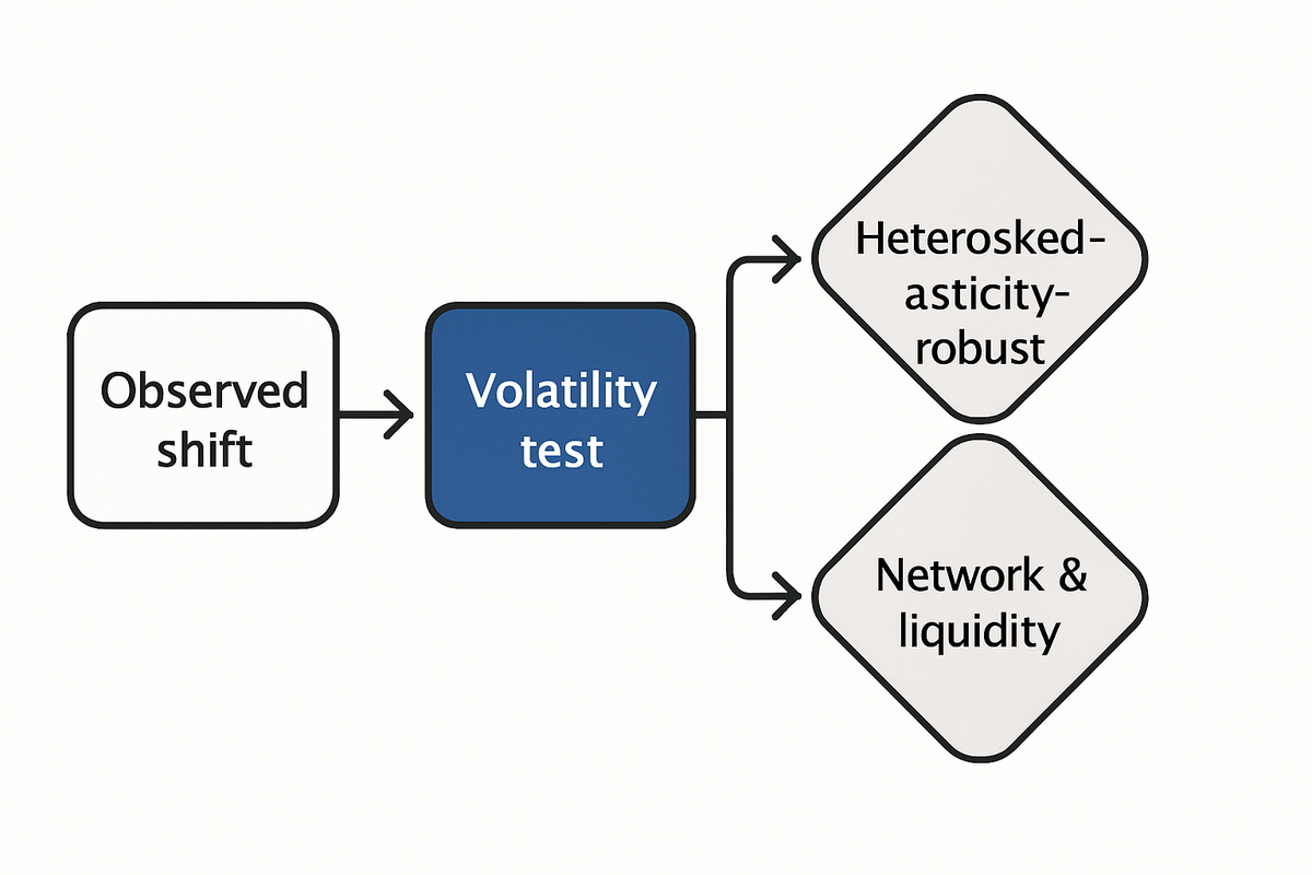
Start with identification. If volatility jumps, simple correlation tests overstate changes because the distribution is not constant across windows. Heteroskedasticity‑robust methods and identification through volatility shifts, as in Rigobon, help separate common‑shock interdependence from extra co‑movement that deserves the label contagion.
Adjust for conditioning. The Federal Reserve’s analysis provides explicit links between conditional and unconditional correlations. Use those relationships to re‑express “crisis‑only” estimates in an unconditional frame before you judge that a breakdown occurred.
Add structure to the map of links. A multi‑layer network approach that blends bilateral bank exposures and CDS spreads gives you contagion channels beyond price co‑moves. That is the point of BIS Working Paper 796 — network effects matter most in crises, and they change loss propagation BIS Working Paper 796.
Use rolling and event‑window templates to calibrate. Large‑sample matrices and rolling correlations, like those in the J.P. Morgan Guide, are not a forecast, yet they define reasonable priors and stress windows. They also anchor decisions about how long a window should be to pick up regime changes without chasing noise.
Finally, track liquidity and flows alongside correlation. Policy analysis in 2025 flagged liquidity spirals and fund‑flow amplifiers as key drivers of tail co‑movements. If your correlation model does not see the order book, you are measuring clouds and missing the rain.
| Tool or lens | What it tests or adds | Typical inputs | When to trust it |
|---|---|---|---|
| Heteroskedasticity‑robust tests | Contagion vs. interdependence | Volatility regimes, global factors | Vol jumps/events |
| Conditional-to-unconditional mapping | Bias from crisis-only samples | Crisis flags, covariances | Post-event audit |
| Rolling/event-window correlations | Regime dependence, timing | Price returns, window rules | Monitoring |
| Multi‑layer network models | Balance‑sheet contagion channels | Exposures, CDS, funding links | System stress |
| Liquidity/flow overlays | Amplifiers of co‑movement | Depth, spreads, fund flows | Stress planning |
| Frequency-aware microstructure checks | Execution risk vs. macro signal | Trade data, venue rules | High-frequency |
Empirical patterns and case studies to anchor strategy
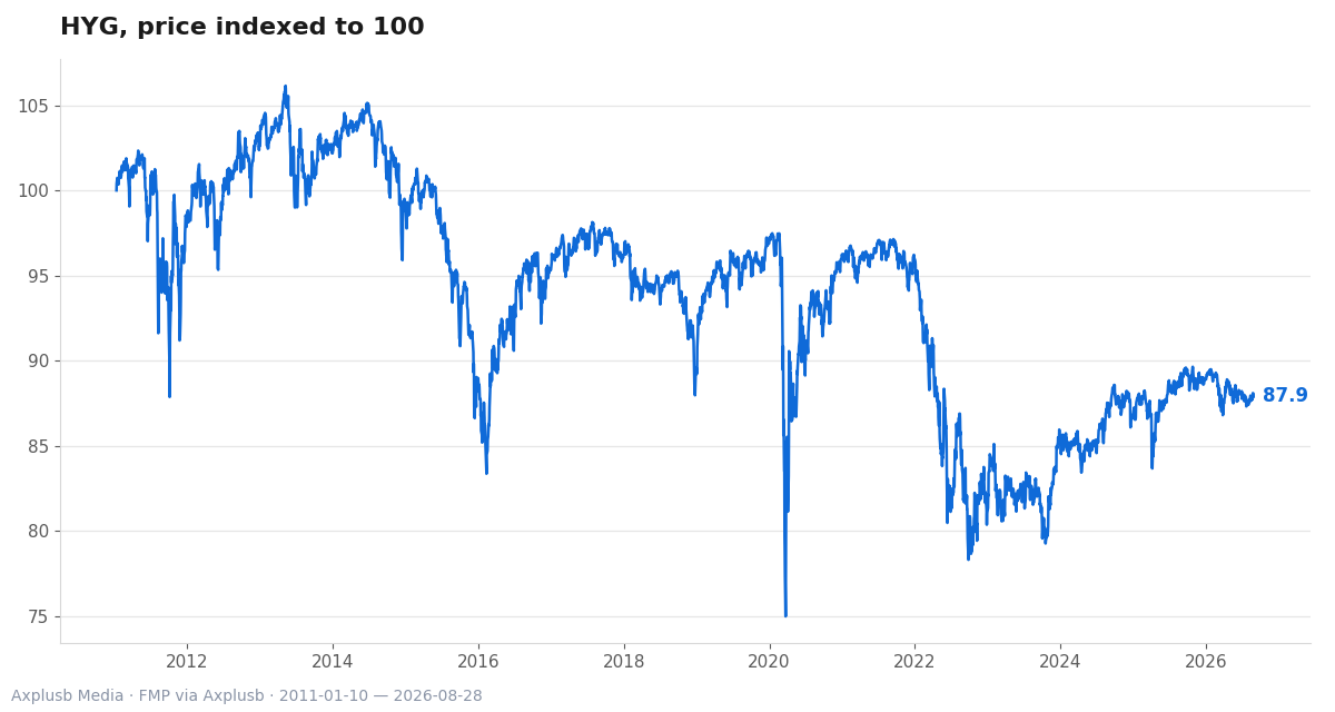
Across cycles, EM correlations shift with the mix of shocks. Global rate moves, commodity cycles and policy actions each pull different strings. The J.P. Morgan matrices show that what looked “low” in one year can look “average” the next, which is a reminder to anchor exposures to a range, not a point.
Network effects raise the stakes when funding tightens. The BIS framework shows how bilateral links and CDS channels can turn a local shock into a system‑wide issue if the network is dense. Correlation rises in the wake of funding stress because balance‑sheet needs align sales across desks.
Diversification within EM is not a free lunch. BlackRock’s note on frontier markets highlights low historical correlation with broad EM and DM indices, yet also flags thin liquidity and political risk. Those two features make any shift faster and wider when exits crowd, which is the textbook path to a correlation jump.
Taken together, the lesson is simple. Historical correlation is a starting point, not a guarantee. Liquidity, balance‑sheet links and the policy backdrop decide the shape of the next move.
Microstructure, liquidity and execution — the frequency dimension
At millisecond horizons, market design matters. The frequent batch auctions proposal, and the evidence behind it, showed how order‑matching rules and arbitrage speed can drive down short‑horizon correlations even when the daily or weekly links hold. Execution slippage in that world is its own risk factor.
Liquidity is the bridge from micro to macro. Policy work in 2025 emphasized that when depth thins and fund flows turn, co‑movements jump across assets and borders. The result is a diversification gap that eats into buffers right when managers lean on them.
The practical outcome is that monitoring must be frequency‑aware. You do not need microsecond tick data for a pension plan, yet you do need to know when local microstructure will undo your hedge. A five‑minute stress window can be the difference between a clean unwind and a bad print.
Counterarguments and limits — what rigorous critics will insist on
The skeptic has a strong case. Once you correct for volatility shifts and common global shocks, many alleged episodes of contagion fade into standard interdependence. Heteroskedasticity‑based identification is not a footnote — it is a filter.
There is also the problem of conditioning. If you run tests only inside crisis days, the math stacks the deck. The Fed’s point about conditional versus unconditional correlation is not subtle, and it is often ignored.
But even if statistical contagion is small, economic co‑movement can still rise in ways that matter. Liquidity, fund flows and balance‑sheet needs can press different holders to act in sync. For risk managers, that sync is enough.
A practical checklist for EM risk managers — monitoring, modelling and governance
A good framework blends statistics and structure. It also sets clear rhythms — what you watch daily, what you re‑calibrate monthly, and when you switch to stress mode. Here is a compact plan you can start tomorrow.
- Run heteroskedasticity‑robust contagion tests and correct for conditional sampling before you label a shift as “real”.
- Maintain rolling correlations and event‑window rules, using large‑sample templates as priors rather than targets.
- Overlay a multi‑layer network map of exposures and CDS links for your key counterparties and markets.
- Track liquidity and fund‑flow indicators next to correlation — thin depth and outflows are early warnings.
- Build frequency‑aware execution limits and stress venues where microstructure can distort short‑horizon hedges.
- Pre‑commit governance triggers for de‑risking when correlation or liquidity crosses set bands.
- Dry‑run the unwind path — who you call, what you sell, and how you pace it across time zones.
Two closing points on process. First, separate detection from action by design — the team that flags a shift should not be the one that sizes the trade. Second, write down the event‑window you will use before the event, and stick to it unless governance says otherwise.
If you need a place to start, adapt the rolling windows and stress dates from the J.P. Morgan Guide, and layer on the network analytics from the BIS framework. Then add qualitative overlays on policy risk and frontier liquidity. That blend matches how correlation actually moves in EMs.
Check how disciplined your portfolio really is. A 30‑minute audit against this list will reveal the gaps that matter.
For deeper tail‑risk design, see our guide on navigating tail risk and connect it to your EM sleeves. If you are building data pipelines for live monitoring, our note on integrating AI into risk management covers alerting and model governance. Political shocks remain a core driver in EM — align your risk playbook with our take on political uncertainty strategies.
Related reading
- Navigating Tail Risk in Uncertain Markets
- Integrating AI into Risk Management Frameworks
- Risk Management and Political Uncertainty