Central banks do not just “set the tone.” They change the cash flows and risks that portfolios face. The question is how to turn policy actions into clear, testable portfolio impacts.
We map the instruments, trace the channels, and give a concrete toolkit you can implement. The aim is simple, if not easy — link balance sheets and rates to the risk and return you own.
What we mean by central‑bank policy and portfolio impact
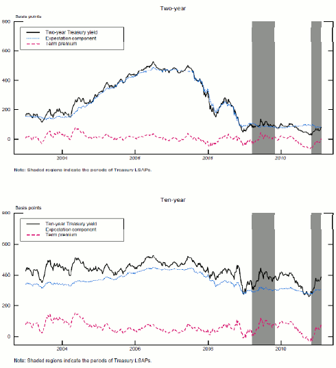
Policy is more than the policy rate. It includes large‑scale asset purchases, balance‑sheet size and composition, and the pace of balance‑sheet “normalization” or QT.
Large‑scale asset purchases lower longer yields by compressing term premia through scarcity and duration channels, as shown by D’Amico et al. (FEDS 2012) with CUSIP‑level evidence. That is the portfolio‑balance channel in action.
Balance‑sheet composition also matters for the system that intermediates risk. A model and calibration in BIS Working Paper No.1173 link balance‑sheet size and duration to intermediary duration risk and resilience, with effects that depend on the debt maturity structure.
Portfolio impact is the measurable change in bond yields and term premia, equity returns and volatility, credit spreads, and the joint behavior of a 60/40. These are the outcomes we target with data and simple regressions.
Why this matters now
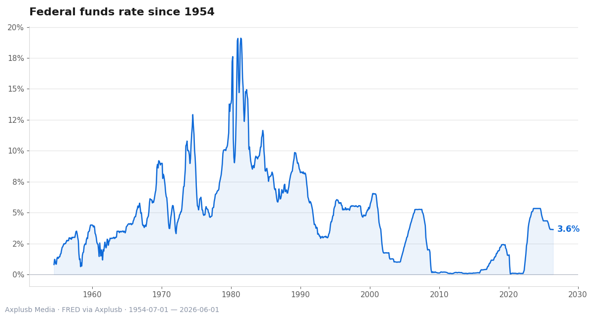
The rate regime has shifted. An institutional view from BlackRock Investment Institute (2023) argues that higher‑for‑longer rates have changed hedging and return tradeoffs, and the 60/40 cushion is weaker.
Balance‑sheet paths are active again. The BIS framework highlights that the effectiveness of balance‑sheet tools depends on the policy rate stance and the structure of public debt, not just on the headline size.
The mix of policy and debt maturity now shapes the term premium and the risk that dealers and funds must absorb. That makes policy settings a first‑order driver of portfolio drawdowns and hedges.
Investors need a way to link policy choices to expected impacts on return, risk, and correlation. Tactical tilts are not optional when the main hedge is less reliable than it was.
Transmission channels: mechanisms, not metaphors
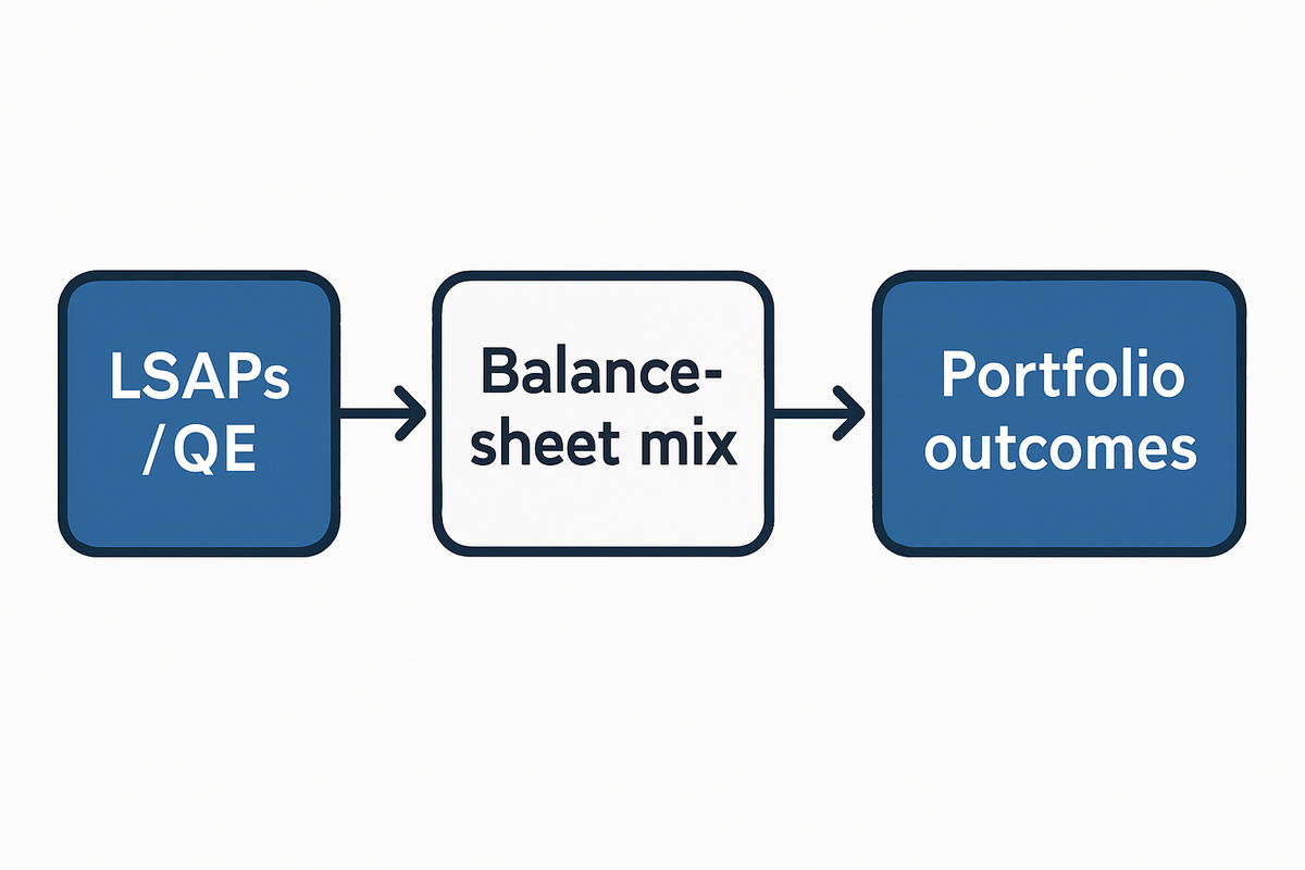
Think in channels. The first is the portfolio‑balance and duration scarcity channel. When a central bank removes duration from the market, the term premium falls, and longer yields drop — this is what FEDS 2012 documents in bond‑by‑bond data.
The second is the intermediary duration risk channel. Balance‑sheet composition can shift duration risk toward or away from dealers and funds. The BIS paper shows how that shift changes resilience and the transmission of conventional policy.
A third idea is refinancing and segmentation. The impact of purchases may differ by asset segment, such as mortgages versus Treasuries. Micro work has proposed this heterogeneity as a testable point, so asset‑level analysis beats a single policy scalar.
How do these channels reach equities and credit. Lower term premia raise the present value of cash flows and can compress credit spreads, while shifts in intermediary balance‑sheet risk can change liquidity and volatility. The direction and size are state‑dependent.
| Channel | Policy lever | Measured object | Expected portfolio effect |
|---|---|---|---|
| Portfolio‑balance / duration scarcity | LSAPs / QE | Term premium on long bonds | Lower yields, higher bond prices, duration‑led gains |
| Intermediary duration risk | Balance‑sheet size and mix | Dealer/fund risk capacity | Liquidity and spread changes, regime‑dependent volatility |
| Conventional rate path | Policy rate and guidance | Short rate and curve slope | Discount rate shifts, equity multiple pressure or relief |
Empirical toolkit: how to measure shocks and responses
Start with event windows around policy announcements and purchase schedules. Calibrate yield moves in basis points using the bond‑level results in FEDS 2012 as your anchor for magnitude.
Then build regime rules on rates and the curve. Use publicly available charts and return histories to classify high versus low rate periods, and to set benchmark returns for simple tests. The goal is to compare like with like across regimes.
For inference, keep it robust. Monetary policy studies often use GMM and Newey‑West errors to guard against weak instruments and serial correlation, so mirror those habits in your asset‑level tests.
Finally, map policy shocks to portfolio metrics. Translate basis‑point shifts into duration‑scaled bond returns, relate curve changes to equity factor moves, and record spread beta for credit.
A note on expectations versus surprises
Policy is a stream, not a point. Distinguish expected path changes from genuine surprises, using announcement windows to isolate the shock.
Expectations do the slow work on valuations. Surprises drive the sharp moves in price and volatility that matter to drawdown control.
Both need attention because the same policy step can have different market effects if it is fully priced or not. Treat the baseline and the shock as separate inputs in your test.
Common misconceptions and pitfalls
Mistake one is to treat QE as a single scalar across assets. The refinancing and segmentation angle suggests the impact can vary by instrument, so do not project Treasury effects onto mortgages or credit.
Mistake two is to assume that market pricing always reflects what central bankers intend. There are times when market belief and policy guidance part ways, which can mute or reverse the near‑term transmission to prices.
Mistake three is to lean only on long‑run equilibrium logic while ignoring the resilience of intermediaries. The BIS framework makes resilience a moving part that changes how policy reaches risk premia.
Mistake four is to keep one hedge for all seasons. The BlackRock view is that higher, stickier rates can blunt the classic 60/40 cushion, which calls for more granular, shorter duration, income‑tilted exposures.
Case studies and quantitative anchors
Bond math first. Use the bond‑level basis‑point impacts on the curve in FEDS 2012 as calibration targets, then translate those into expected bond return changes with your portfolio duration profile.
Next, set up rate regimes. Define high and low rate states and record average bond, equity, and credit returns for each state across your sample. The rule can be simple, but it must be explicit and stable.
For portfolios, build a plain 60/40 and a dynamic tilt version. The tilt follows the BlackRock guidance to use shorter duration and more granular income when rates are high and central banks are shrinking balance sheets.
Then test a balance‑sheet sensitivity. Vary the size and duration of a notional central‑bank portfolio and run the implied change in term premia through your bond sleeve, and through the discount rates you use in equity models.
| Use case | Input | Calibration anchor | Portfolio output |
|---|---|---|---|
| Event study on QE | Announcement window bp move | FEDS 2012 CUSIP‑level yield shifts | Duration‑scaled bond return, term‑premium beta |
| Regime backtest | Rate level and curve slope | Public charts and return history | 60/40 vs tilt, drawdown and Sharpe |
| QT stress | Balance‑sheet size and duration | BIS model of intermediary risk | Spread change, liquidity proxy, hedge hit rate |
Alternative views, limits and the role of sentiment
Balance‑sheet effects are model dependent. The BIS paper shows that the same balance‑sheet move can have different outcomes when debt maturity or the policy rate stance changes.
Market belief can diverge from policy messages. In those episodes, prices may move with risk appetite rather than with guidance, so attribution to policy alone will mislead.
Identification is hard in reduced‑form tests. Use multiple windows and instruments, and compare results across sub‑samples, to avoid chasing noise that looks like a policy effect.
Do not force a single story. Keep channels and regimes separate in your code, then combine them only at the portfolio layer, where tradeoffs are clear.
Practical playbook for portfolio teams
Build a parsimonious dataset. Include policy rate, term premium proxy, central‑bank balance‑sheet size and an estimate of its duration, curve slope, and a debt maturity index.
Calibrate the bond block with basis‑point anchors from FEDS 2012. Convert yield changes into expected price moves using your actual key‑rate durations.
Classify regimes and run two backtests: a static 60/40 and a rule‑based tilt that shortens duration and adds income in high‑rate states, following BlackRock’s guidance. Compare drawdowns, hedge hit‑rates, and rebalancing costs.
Stress the system. Shock balance‑sheet size and composition, as in BIS WP 1173, then track how spread beta, liquidity proxies, and volatility respond in your holdings.
- Variables: policy rate, curve slope, term premium proxy, balance‑sheet size, balance‑sheet duration, debt maturity mix.
- Tests: event windows, regime backtests, spread beta, liquidity sensitivity.
- Scenarios: LSAP on, QT on, higher‑for‑longer rates, change in debt maturity profile.
- Outputs: expected return shift, volatility change, hedge effectiveness, drawdown paths.
Check how disciplined your portfolio really is. Run the event and regime tests on your last three years, and write down the rules you would have followed.
Appendix: a reproducible workflow
Step one — data and charts. Pull policy rates, curve data, and return histories from the same sources you use to brief your committee, so your rules match your charts.
Step two — event windows. Code narrow windows around policy days and purchase schedule announcements. Measure basis‑point moves, then translate them into returns with key‑rate and effective duration.
Step three — regressions. Regress bond and equity returns on your policy shock variables and regime dummies. Use robust errors to keep inference stable when noise is high.
Step four — portfolio synthesis. Combine the bond and equity blocks into your base mix, then add a tilt that reacts to regime states and balance‑sheet shocks. Record turnover and any change in liquidity risk.
Two diagnostic plots make the process tangible. First, a ladder of expected bond return per 10 bp of curve move for your holdings. Second, a line that shows how the 60/40 hedge hit‑rate changes across rate regimes.
Asset heterogeneity is your last mile. Run sector‑level and credit‑quality splits rather than treating policy as a single number that hits all assets in the same way.
If you use models to make these rules repeatable, make sure your tools do not overfit the event windows. Practical machine learning can help you select stable features — see how this sits with AI in portfolio optimization.
Conclusion and what to watch next
Policy is now a portfolio risk you can and should measure. Balance‑sheet paths and higher‑for‑longer rates alter the hedge that many investors took for granted.
The channels are clear enough to model. Term premia move when duration is scarce, and intermediary resilience shapes how shocks reach spreads and volatility, as laid out in BIS WP 1173.
The practical stance is calm and firm. Monitor balance‑sheet composition, recalibrate duration bets, test the 60/40 hedge by regime, and keep an eye on liquidity.
The market’s market is changing too. Digital rails and new instruments could change how policy transmits, as we discussed in our CBDC analysis and in our tokenized assets piece.
Stress your playbook before the next meeting. If you can explain how 25 basis points or a balance‑sheet tweak hits your holdings, you are ready.
Related reading
- The Impact of Central Bank Digital Currencies on Traditional Portfolio Strategies
- The Future of Tokenized Assets: Impact on Portfolio Diversification Strategies
- The Impact of AI on Portfolio Optimization: What Investors Should Consider