A point-in-time backtest across four horizons finds no predictive edge for EV/EBITDA inside the S&P 500, with the effect running opposite to the value hypothesis.
The starting hypothesis was straightforward: stocks trading cheap on EV/EBITDA, measured as a percentile rank rather than an absolute multiple, should earn higher subsequent returns, and a portfolio built on that filter should beat the S&P 500.
The test was designed to give a formal answer rather than a best-case historical return: point-in-time data, no survivorship bias, run separately on the historical composition of the S&P 500 and on a broader investable universe, ending in a verdict on whether the factor has a standalone edge worth building on.
Key figures of the study
Summary
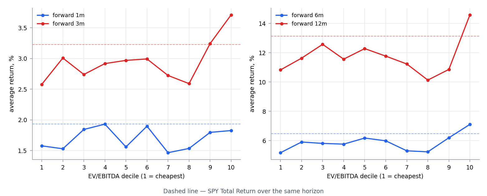
The results run the other way from the hypothesis. The rank correlation between cheapness and forward returns is negative at every horizon tested — -0.010 at one month, -0.016 at one quarter, -0.015 at six months and -0.015 at one year — and the cheapest decile returned 10.83% over twelve months against 14.59% for the most expensive decile.
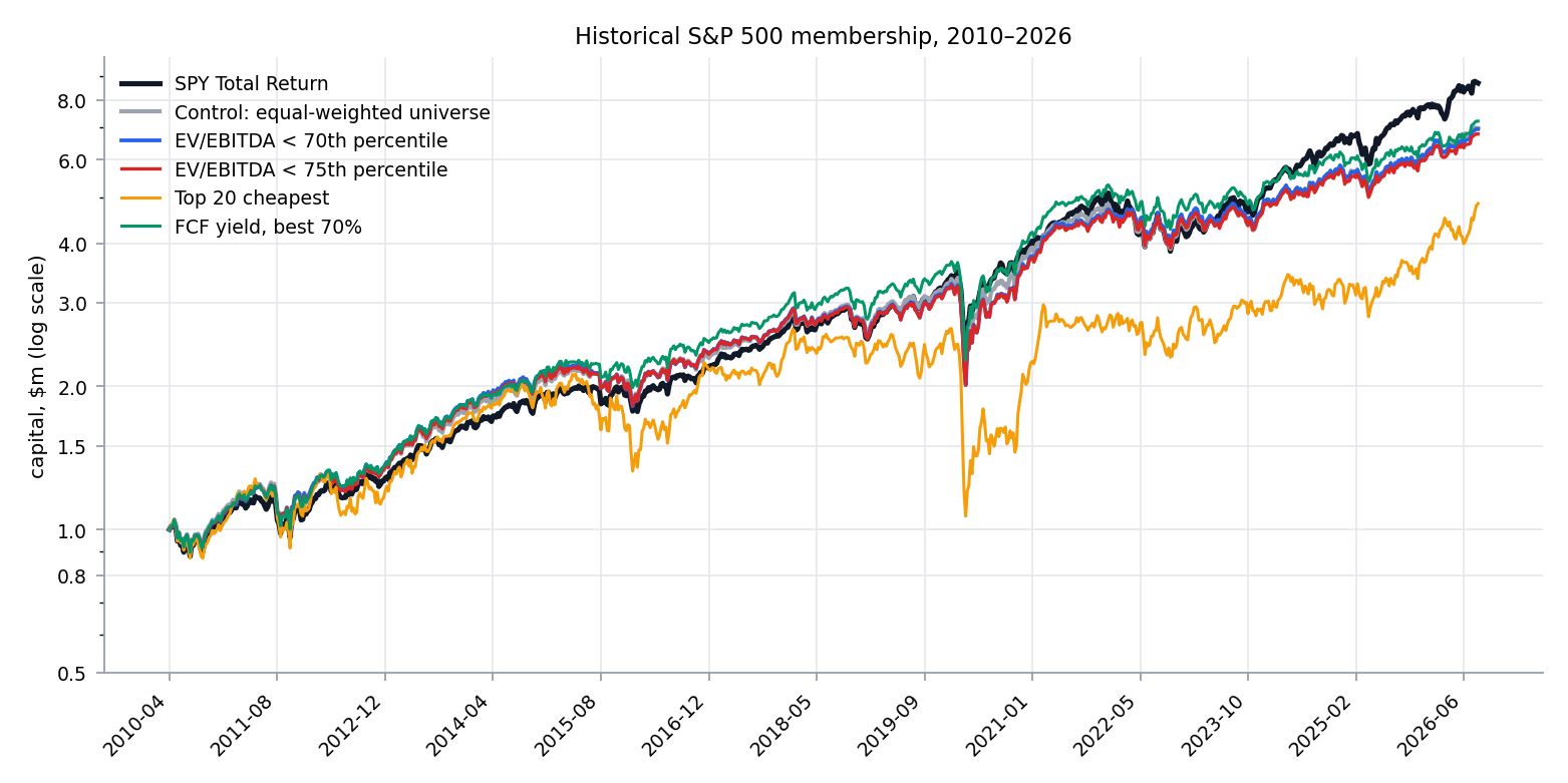
No percentile threshold beat the index, and the comparison that matters is against an equal-weight, no-filter control rather than the cap-weighted S&P 500: the EV/EBITDA-under-70th-percentile portfolio returned 12.46% a year against 12.47% for the same universe held with no filter at all — a difference of one hundredth of a percentage point.
| Portfolio | CAGR | Excess vs SPY TR | Sharpe | Max DD | Information ratio |
|---|---|---|---|---|---|
| SPY Total Return | 14.06% | — | 0.70 | −33.7% | — |
| EV/EBITDA < 50th percentile | 12.65% | −1.41 pp | 0.59 | −41.9% | −0.18 |
| EV/EBITDA < 60th percentile | 12.69% | −1.38 pp | 0.61 | −40.1% | −0.19 |
| EV/EBITDA < 65th percentile | 12.53% | −1.53 pp | 0.61 | −39.5% | −0.22 |
| EV/EBITDA < 70th percentile (main hypothesis) | 12.46% | −1.60 pp | 0.61 | −38.8% | −0.24 |
| EV/EBITDA < 75th percentile (alternative) | 12.29% | −1.77 pp | 0.60 | −38.5% | −0.27 |
| EV/EBITDA < 80th percentile | 12.26% | −1.80 pp | 0.60 | −38.6% | −0.28 |
| Top-20 cheapest | 10.13% | −3.93 pp | 0.31 | −59.9% | −0.23 |
| Top-10 cheapest | 5.34% | −8.72 pp | 0.12 | −68.6% | −0.42 |
| Top-5 cheapest | 6.35% | −7.71 pp | 0.14 | −72.3% | −0.31 |
| Control: entire eligible universe equal-weighted | 12.47% | −1.60 pp | 0.62 | −36.8% | −0.32 |
| Period | 50 | 60 | 65 | 70 | 75 | 80 |
|---|---|---|---|---|---|---|
| Training 2010–2016, excess CAGR, pp | +1.19 | +1.08 | +1.08 | +1.18 | +1.14 | +0.90 |
| Training, information ratio | +0.28 | +0.30 | +0.31 | +0.36 | +0.36 | +0.30 |
| Validation 2017–2020, excess CAGR, pp | −6.03 | −4.54 | −4.36 | −4.46 | −4.70 | −4.62 |
| Validation, information ratio | −0.59 | −0.50 | −0.51 | −0.55 | −0.61 | −0.63 |
| Final OOS 2021–2026, excess CAGR, pp | −3.89 | −4.31 | −4.86 | −4.91 | −5.10 | −5.02 |
Hypothesis and precise filter definition
The filter is defined as a percentile cut within each rebalancing date’s cross-section, not as an absolute EV/EBITDA level — an absolute reading made little sense given that the S&P 500 median multiple rose from 9.3 in 2010 to 15.9 in 2026.
The primary test used the 70th percentile, with the 75th percentile and a range of alternative thresholds checked as sensitivity, alongside concentrated top-name portfolios and an equal-weight, no-filter control used to isolate the filter’s own contribution.
Universes
The core test uses the historical composition of the S&P 500 across 66 quarterly dates from March 2010 to June 2026, covering 814 unique names over the period, with between 302 and 428 names ranked by EV/EBITDA on any given date.
Cross-sectional analysis: does the factor work on its own
Before looking at any portfolio, the analysis asks a simpler question: is there any relationship at all between EV/EBITDA and subsequent returns? The rank correlation is essentially zero and, where it differs from zero, runs the wrong way — the cheapest decile underperformed the most expensive decile by 3.76 percentage points a year, and the ranking of deciles by return does not move monotonically with the ranking by valuation.
The pattern holds when EV is defined differently and when financials are excluded, and one further check stands out: companies with negative EBITDA, which the multiple cannot rank at all, returned 19.9% a year — well above the index and above every decile — a reminder that the multiple’s built-in exclusion is itself a form of stock selection.
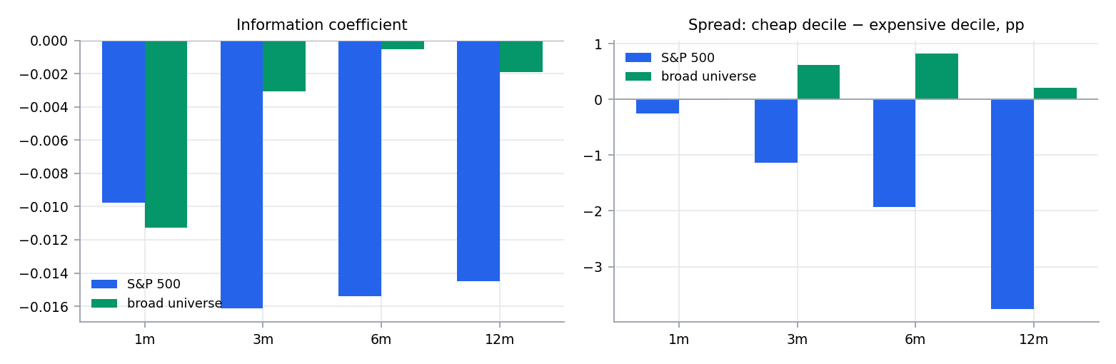
| Horizon | Average IC | Median IC | t-statistic | Share of dates with IC > 0 | Dates |
|---|---|---|---|---|---|
| 1 month | −0.0098 | −0.0043 | −0.48 | 48.5% | 66 |
| 3 months | −0.0161 | −0.0344 | −0.81 | 46.2% | 65 |
| 6 months | −0.0154 | +0.0014 | −0.73 | 51.6% | 64 |
| 12 months | −0.0145 | −0.0113 | −0.65 | 46.8% | 62 |
| Decile | Average 12m | Median 12m | Beat SPY, share of dates |
|---|---|---|---|
| 1 (cheap) | 10.83% | 9.49% | 32.3% |
| 2 | 11.64% | 9.53% | 37.1% |
| 3 | 12.58% | 10.62% | 48.4% |
| 4 | 11.57% | 10.12% | 38.7% |
| 5 | 12.29% | 10.19% | 48.4% |
| 6 | 11.77% | 10.65% | 41.9% |
| 7 | 11.24% | 9.64% | 37.1% |
| 8 | 10.14% | 9.07% | 40.3% |
| 9 | 10.86% | 10.35% | 37.1% |
| 10 (expensive) | 14.59% | 13.84% | 56.5% |
| SPY Total Return | 13.13% | — | — |
| Quartile | Average return 12m |
|---|---|
| 1 (cheap) | 11.66% |
| 2 | 11.89% |
| 3 | 11.38% |
| 4 (expensive) | 12.07% |
| Variant | IC 12m | Spread of extreme deciles 12m | Decile 1 | Decile 10 |
|---|---|---|---|---|
| Main (EV = MCap + Debt − Cash) | −0.0145 | −3.76 pp | 10.83% | 14.59% |
| EV with minority interest and preferred shares | −0.0129 | −3.70 pp | 10.75% | 14.44% |
| Financial sector included in ranking | −0.0153 | −2.97 pp | 11.40% | 14.38% |
| Basket | Average return 12m | ||
|---|---|---|---|
| EBITDA ≤ 0 | (excluded from factor) | 19.87% | |
| EV ≤ 0 | (excluded from factor) | 13.33% | |
| Entire ranked universe (average across deciles) | 11.75% | ||
| SPY Total Return | 13.13% |
Backtest on the historical S&P 500 composition
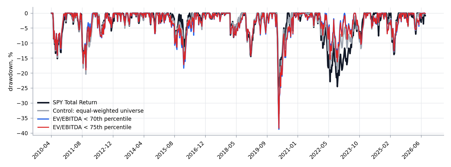
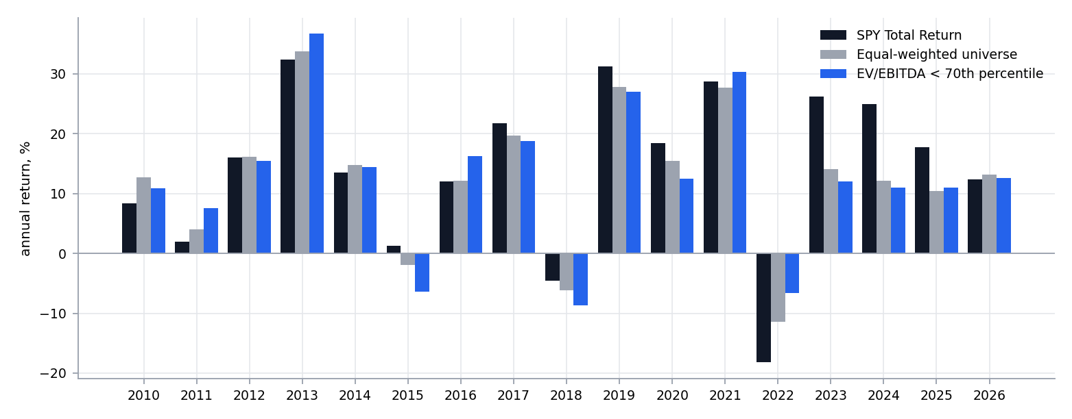
Running the filter as an actual portfolio from April 2010 to September 2026, with quarterly rebalancing, confirms the cross-sectional finding: the filter’s own contribution, measured against the equal-weight control rather than the index, hovers around zero across sub-periods, rolling three-year windows and independent year-by-year tests, with only 8 of 17 calendar years showing a positive result.
The one year the filter clearly won was also the one year expensive stocks broadly fell — the profile of a value factor that pays off only when growth stocks sell off, not a standing source of return.
| Metric | SPY TR | EV/EBITDA <70 | EV/EBITDA <75 | EW universe | Expensive >70 | Top-20 cheap |
|---|---|---|---|---|---|---|
| Total Return | 763.6% | 585.2% | 568.5% | 585.4% | 585.3% | 385.9% |
| CAGR | 14.06% | 12.46% | 12.29% | 12.47% | 12.46% | 10.13% |
| Annual volatility | 17.12% | 17.15% | 17.02% | 16.94% | 18.58% | 25.87% |
| Sharpe | 0.70 | 0.61 | 0.60 | 0.62 | 0.56 | 0.31 |
| Sortino | 0.87 | 0.77 | 0.76 | 0.77 | 0.72 | 0.42 |
| Max Drawdown | −33.7% | −38.8% | −38.5% | −36.8% | −34.4% | −59.9% |
| Calmar | 0.42 | 0.32 | 0.32 | 0.34 | 0.36 | 0.17 |
| Alpha (annual) | — | −0.67 | −0.81 | −0.96 | −2.08 | −5.41 |
| Beta | — | 0.92 | 0.92 | 0.95 | 1.04 | 1.12 |
| Tracking error | — | 6.80% | 6.57% | 4.99% | 5.39% | 17.45% |
| Information Ratio | — | −0.24 | −0.27 | −0.32 | −0.30 | −0.23 |
| Monthly hit rate vs SPY | — | 48.2% | 46.7% | 44.7% | 47.7% | 49.2% |
| Win/loss (average outperformance / underperformance) | — | 0.90 | 0.92 | 0.95 | 0.89 | 0.98 |
| Turnover per rebalance | — | 18.2% | 16.2% | 6.8% | 35.0% | 64.9% |
| Average holding period | — | 682 days | 734 days | 1 309 days | 250 days | 177 days |
| Positions at period end | 1 | 295 | 317 | 421 | 126 | 20 |
| Total trades | — | 4 178 | 3 971 | 2 463 | 4 441 | 1 553 |
| Share of time in market | — | 99.98% | 99.9% | 99.9% | 100% | 99.8% |
| Average cash share | — | 2.30% | 2.58% | 3.06% | 0.0% | 0.24% |
| Costs over period | — | 3.57% of capital | 3.11% | 1.20% | 7.20% | 9.40% |
| Threshold | Training, vs EW | Validation, vs EW | Final OOS, vs EW |
|---|---|---|---|
| 50 | +0.35 pp | −3.44 pp | +0.57 pp |
| 60 | +0.25 | −1.95 | +0.15 |
| 65 | +0.24 | −1.77 | −0.40 |
| 70 | +0.34 | −1.87 | −0.45 |
| 75 | +0.30 | −2.11 | −0.64 |
| 80 | +0.06 | −2.03 | −0.57 |
| Year | SPY TR | EW universe | EV/EBITDA < 70 | Excess vs SPY |
|---|---|---|---|---|
| 2010 | 8.40% | 12.66% | 10.86% | +2.46 |
| 2011 | 1.89% | 3.98% | 7.58% | +5.69 |
| 2012 | 15.99% | 16.09% | 15.49% | −0.50 |
| 2013 | 32.31% | 33.69% | 36.64% | +4.33 |
| 2014 | 13.46% | 14.74% | 14.35% | +0.89 |
| 2015 | 1.25% | −1.93% | −6.45% | −7.70 |
| 2016 | 12.00% | 12.08% | 16.25% | +4.25 |
| 2017 | 21.70% | 19.62% | 18.76% | −2.94 |
| 2018 | −4.56% | −6.19% | −8.66% | −4.10 |
| 2019 | 31.22% | 27.78% | 27.01% | −4.21 |
| 2020 | 18.37% | 15.45% | 12.48% | −5.89 |
| 2021 | 28.74% | 27.61% | 30.27% | +1.53 |
| 2022 | −18.17% | −11.43% | −6.58% | +11.59 |
| 2023 | 26.19% | 14.05% | 12.04% | −14.15 |
| 2024 | 24.89% | 12.16% | 10.98% | −13.91 |
| 2025 | 17.72% | 10.39% | 10.92% | −6.80 |
| 2026 (6 mo.) | 12.31% | 13.13% | 12.56% | +0.25 |
| Portfolio | Share of windows with positive excess | Average excess | Worst window | Best window |
|---|---|---|---|---|
| EV/EBITDA < 70 | 32.9% | −6.23 pp | −49.97 pp | +26.32 pp |
| EV/EBITDA < 75 | 33.5% | −6.78 pp | — | — |
| EW universe | 32.3% | −6.57 pp | −45.79 pp | +10.84 pp |
| 2010 | 2011 | 2012 | 2013 | 2014 | 2015 | 2016 | 2017 | 2018 |
|---|
| EV/EBITDA < 70 | +2.5 | +3.3 | +2.2 | +2.0 | −1.2 | −8.5 | −1.0 | −2.3 | −3.2 | |||||
|---|---|---|---|---|---|---|---|---|---|---|---|---|---|---|
| EW universe | +4.3 | +0.2 | +1.6 | +0.4 | −0.5 | −5.2 | −2.7 | −2.1 | −1.5 | |||||
| 2019 | 2020 | 2021 | 2022 | 2023 | 2024 | 2025 | 2026 | |||||||
| EV/EBITDA < 70 | −3.8 | +9.5 | −5.4 | +8.7 | −8.3 | −9.2 | −11.8 | −6.7 | ||||||
| EW universe | −4.2 | +7.5 | −3.2 | +5.7 | −7.4 | −9.2 | −10.2 | −5.8 |
Formal threshold-selection protocol
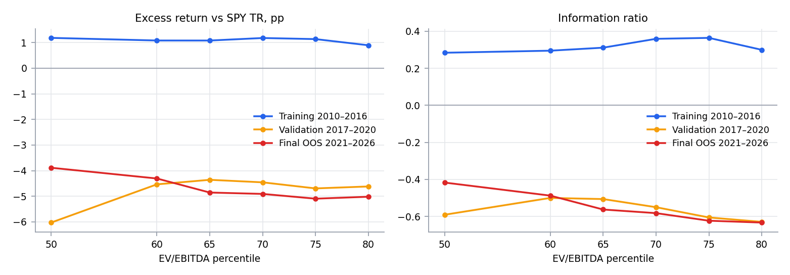
To keep the threshold choice honest, the selection rule was written down and locked before any result was seen: a threshold had to show a positive risk-adjusted excess return on two separate historical periods, with neighbouring thresholds also passing, before it could be selected — and the final holdout period could not be used in the selection at all.
No threshold passed. On the earliest of the two periods every threshold tested actually looked positive, which is exactly the pattern that would have been mistaken for a robust factor had the periods not been separated in advance; the later period reversed it, and the untouched holdout period repeated the same negative sign.
| Period | Bounds | Rebalances |
|---|---|---|
| Training / Research | 01.01.2010 — 31.12.2016 | 28 |
| Validation | 01.01.2017 — 31.12.2020 | 16 |
| Final Out-of-Sample | 01.01.2021 — 30.06.2026 | 22 |
| Threshold | Training: excess CAGR / IR | Validation: excess CAGR / IR | Passed? |
|---|---|---|---|
| 50 | +1.19 pp / +0.28 | −6.03 pp / −0.59 | no |
| 60 | +1.08 / +0.30 | −4.54 / −0.50 | no |
| 65 | +1.08 / +0.31 | −4.36 / −0.51 | no |
| 70 | +1.18 / +0.36 | −4.46 / −0.55 | no |
| 75 | +1.14 / +0.36 | −4.70 / −0.61 | no |
| 80 | +0.90 / +0.30 | −4.62 / −0.63 | no |
| Threshold | Final OOS: CAGR | Excess vs SPY | IR | Sharpe | Max DD |
|---|---|---|---|---|---|
| 50 | 10.32% | −3.89 pp | −0.42 | 0.54 | −18.1% |
| 60 | 9.90% | −4.31 | −0.49 | 0.52 | −18.1% |
| 65 | 9.35% | −4.86 | −0.56 | 0.49 | −18.0% |
| 70 | 9.30% | −4.91 | −0.58 | 0.49 | −17.7% |
| 75 | 9.11% | −5.10 | −0.62 | 0.48 | −18.3% |
| 80 | 9.19% | −5.02 | −0.63 | 0.48 | −18.9% |
| SPY TR over period | 14.21% | — | — | — | — |
Biases and limitations
Several data limitations remain, and all identified biases point the same direction: they inflate the result rather than mask a real effect. Restated financial figures, the treatment of acquired companies and the use of annual rather than trailing-twelve-month accounting each work in the filter’s favour, and the finding still comes out negative.
The study covers a single market and a single sixteen-year period — one that was historically strong for richly-valued growth stocks — so the conclusion describes EV/EBITDA in US equities over 2010–2026 rather than a universal statement about value investing.
| Bias | How closed | ||
|---|---|---|---|
| Look-ahead in financial statements | filter by | acceptedDate | , § 3.2 |
| Look-ahead in prices and market cap | series truncated by date, forward returns only forward-looking | ||
| Look-ahead via ready-made FMP multiples | no derived datasets used, EV and EBITDA computed in-house | ||
| Look-ahead via index composition | members_on(T) | , § 3.3 | |
| Survivorship bias in S&P 500 | historical log of index changes | ||
| Survivorship bias in broad universe | delisted names included, § 10.1 | ||
| Equal-weight effect mistaken for factor effect | equal-weighted control, § 2.3 | ||
| Threshold overfitting | protocol fixed before the run, § 8 | ||
| Sector bet | sector-neutral variant, § 9.2 | ||
| Size bet | cap-based cuts vs. own-bucket control, § 9.4 | ||
| Sensitivity to EV definition | variant with minority interest and preferred shares, § 6.4 | ||
| Sensitivity to excluding financials | variant with their inclusion, § 6.4 |
Conclusion
Taken together, the evidence rules out a genuine factor and rules out a case of overfitting alike: no threshold beats the index or the equal-weight control on any of the three periods tested, and the cross-sectional relationship runs opposite to the hypothesis throughout. The classification is no edge, and the verdict is not to integrate the factor into any live process.
EV/EBITDA’s inverse is already used at a modest weight within an existing internal valuation framework, and nothing here supports increasing that weight. Two exploratory configurations showed isolated promise, but neither passed the pre-registered selection criteria and both were built on portfolios of only a handful of stocks — too small to distinguish signal from noise. They stand as hypotheses for future testing, not as findings.
EV/EBITDA, tested as a percentile filter across sixteen years of point-in-time data, shows no standalone predictive power in the S&P 500 and, if anything, points the wrong way. The classification is no edge, and the verdict is not to integrate it into any production process.
That is not the same as finding nothing. The exercise shows why an equal-weight control and pre-registered test periods are indispensable safeguards — without them, this same data would have told a convincing but false story of a working value factor.
Every figure, table and chart in this article comes from Axplusb in-house quantitative research, 09.2026. Nothing has been recalculated for publication.
This article is an editorial summary of an in-house quantitative research report. It is information, not investment advice, and it is not a personal recommendation: the figures are as of the date of the underlying research.