Machine learning promised sharper signals and broader data. It also made backtesting both harder and more important. The methods are not an add‑on to classical tests, they change what “validated” even means.
Defining ML backtesting in quantitative strategies
Backtesting with machine learning replaces a fixed rule with an adaptive mapping from inputs to trades. The model learns patterns from history, then updates, selects hyperparameters, and sometimes refits on a rolling basis. That loop breaks the simple in‑sample versus out‑of‑sample split that factor tests once relied on. It demands time‑aware validation and careful control of model choice.
A broad survey of practice highlights the point. In finance, samples are short, signals are weak and regimes shift. This is why walk‑forward evaluation, rolling windows and regularization show up as core advice in the AQR overview of financial ML practice, which also stresses the small‑data constraint faced by most investors AQR’s survey of financial machine learning.
The validation problem also includes a cost of selection. We test many model ideas, hyperparameters and features, then keep the best one. The literature on the Probability of Backtest Overfitting formalized this risk and proposed ways to measure it. It also reframed backtesting length and partition design as part of the model itself, not a neutral choice.
If you are working on signal rotation, the challenge is concrete. A rule that looks stable can be an artifact of selection, not an edge. See how we handled this tension in Leveraging Machine Learning for Enhanced ETF Rotation Strategies.
Why this matters now: data, compute and model complexity
Two trends drive urgency. First, adoption is broad in policy and markets, which raises the bar for governance. A central bank survey documents wide use of ML, along with concerns around data quality, representativeness and model risk management BIS Working Paper No 930 on big data and machine learning.
Second, the data menu and compute budget have grown, yet the effective sample for many signals is still short. The AQR survey notes that financial applications often face small data and noisy labels, which forces care in cross‑validation and model choice AQR’s survey of financial machine learning.
Practitioners echo this tension. In macro settings, teams pool cross‑sections, lean on domain priors and use regularization to keep models from learning noise. That framing fits the backtesting problem as well, because the validation choices must match the data’s shape and the economic story.
Backtesting therefore sits at the junction of modeling and governance. The statistical stance must be strict and the documentation must travel with the code. The combination is what keeps research from drifting into a one‑off, lucky run.
The core failure modes: overfitting, data‑snooping, survivorship and model risk
Overfitting is the headliner. Try enough models on a finite sample and one will look great by chance. The framework for the Probability of Backtest Overfitting defines this problem and ties it to the design of the testing partitions. It also motivates tools like time‑aware cross‑validation and deflated performance metrics.
Data‑snooping is the cousin of overfitting. We peek, then adapt the test to the data, often without writing that step down. Adding or dropping features after each run amplifies selection on noise. Formal treatments argue for methods that account for the number of tries, not just the winner’s score.
Survivorship bias and sample design complete the picture. Dropping dead tickers or using an index that reconstitutes silently inflates past performance. Short effective sample length makes this worse, because a few quarterly events can drive most of the measured edge.
Model risk binds these into a governance task. The BIS survey highlights concerns about data quality and representativeness, which feed the same failure modes in backtests BIS Working Paper No 930 on big data and machine learning.
The practitioner’s toolkit: walk‑forward, rolling CV, penalization and deflation
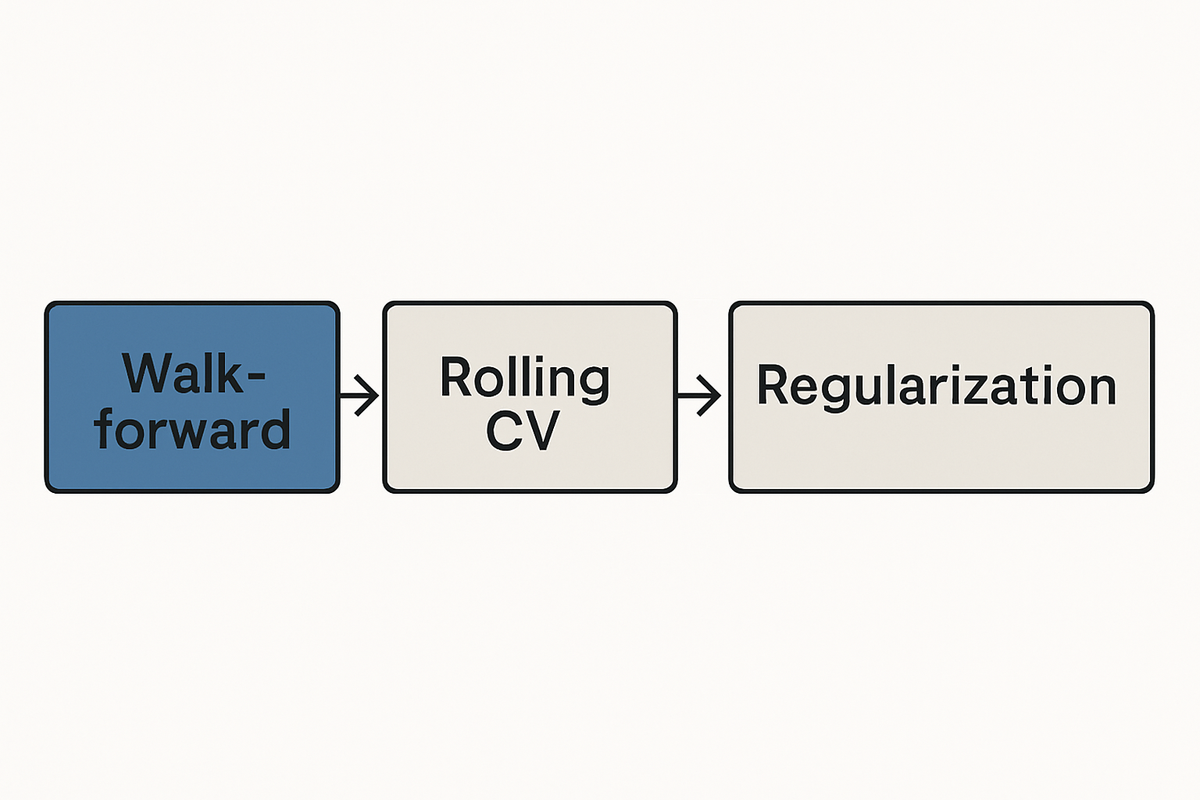
Robust backtesting starts with the split. A rolling or walk‑forward setup trains on a moving window and tests on the next slice, then rolls again. The AQR survey describes this as a practical default given the small‑sample and non‑stationary nature of financial data AQR’s survey of financial machine learning.
Time‑aware cross‑validation extends the idea. Instead of random folds, each fold respects ordering and uses past to predict future. This aligns the learning task with reality and helps control optimistic bias from leakage. It also provides multiple out‑of‑sample checks for the same model family.
Penalization belongs in the selection step. Regularization shrinks unstable parameters and rewards simpler explanations that still fit. When we present a Sharpe or hit rate, a deflated or penalized version acknowledges model search and noise. The goal is not to depress everything, it is to downgrade the easy wins that came too cheap.
Below is a compact map for the toolkit.
| Technique | Purpose in backtesting | Primary guidance |
|---|---|---|
| Walk-forward evaluation | Mimic live re-training and deployment cadence | AQR survey on rolling setups |
| Time-aware cross-validation | Reduce leakage and optimistic bias | AQR survey on small data CV |
| Regularization | Control variance and shrink unstable fits | AQR survey on regularization |
| Deflated performance metrics | Account for model search inflation | PBO framework and related work |
If your strategy must adapt to fast macro swings, this structure matters. We explored similar safeguards in Advanced Backtesting Techniques for Quantitative Strategies in Uncertain Times.
Advanced statistical fixes: CSCV, covariance penalties and TLS adjustments
Combinatorially‑Symmetric Cross‑Validation was designed to estimate the chance that a backtest is the best only by luck. It builds many time‑respecting splits, evaluates each candidate and then measures how often the winner fails out of sample. That ratio approximates the Probability of Backtest Overfitting as defined in the foundational work.
Covariance‑penalty corrections attack the optimism in estimated performance. The idea is to subtract a penalty that rises with model complexity and data noise. Evidence suggests that these penalties, along with Total Least Squares style adjustments, can lower the gap between in‑sample and forward results. They do not fix a bad idea, they make the score more honest.
These methods are not heavy to implement. CSCV can be layered on a rolling workflow. Penalized estimates can be reported next to the raw figures as a standing rule. The main cost is compute time, and that cost is small next to a painful live drawdown.
Finally, they teach humility. If the penalized Sharpe falls to a level that fails your hurdle, you should treat the edge as unproven. That decision is cheaper to make on paper than in production.
Synthetic data and generative stress‑testing: promise and limits
Generative models offer a different lens. A recent study proposes using a GAN with sequence models to create synthetic price paths, then testing a strategy on those alternate histories to detect overfitting a GAN-based approach to synthetic backtesting on arXiv.
The intuition is simple. If a strategy only wins on the one path we observed, it may fail on nearby paths drawn from a learned distribution. A diverse set of synthetic histories can expose that fragility. It can also surface cases where the model relies too much on a single market phase.
There are limits. Synthetic data are only as rich as the model and training sample allow. Industry analysis warns that these generators can miss real regime shifts and market microstructure complexity, so they cannot remove the core uncertainty of forecasting. Treat them as stress tests, not replacements for real out‑of‑sample time.
Use clear rules here. Specify which statistics the GAN must match and which failure modes you want to probe. Report results with the same caution you would apply to a small backtest. A pass on fake data is a necessary condition, not a sufficient one.
Institutional lens: governance, data quality and model risk controls
Backtesting lives inside a governance stack. Central banks report strong interest in ML, yet cite data quality, representativeness and oversight as key concerns for model risk BIS Working Paper No 930 on big data and machine learning.
That list translates well to the buy side. Provenance tells you how the data were built and revised. Representativeness asks whether the training sample covers the use case. Oversight requires a clear record of model versions, parameter choices and validation outcomes.
Practitioners also endorse domain priors. In macro ML, teams combine cross‑sections, encode economic structure and apply regularization to reduce overfitting in sparse data. The message for backtesting is to write the prior into the design, not only into the model. Your splits, penalties and metrics should reflect how the signal is expected to work.
This is not red tape. A clean pipeline and a written validation plan stop the quiet creep of data‑snooping and selection on the dependent variable. They also help when explaining a drawdown to a risk committee.
Empirical evidence and practitioner case studies
The thread across studies and practice is consistent. The AQR survey documents that rolling windows, walk‑forward tests and regularization are standard tools for financial ML, because the data are short and non‑stationary AQR’s survey of financial machine learning.
In macro, practitioner guides report that pooling cross‑sections and adding domain priors help with sparse labels and overfitting. Those choices also ease backtest optimism, because they constrain the hypothesis space. You get fewer degrees of freedom for the same economic exposure.
Formal methods add power. Work on covariance‑penalties and related adjustments shows empirical gains in closing the in‑sample to out‑of‑sample gap. And the GAN approach illustrates how synthetic paths can reveal when a strategy wins only because a single history cooperated a GAN-based approach to synthetic backtesting on arXiv.
None of these erase uncertainty. They change the base rate and give you more honest odds. That is what a backtest should do.
Counterarguments and sober limits: no panacea for regime change
It is tempting to hope for a final fix. There is none. Synthetic histories cannot anticipate structural breaks that never occurred in the training data. They also struggle with market structure details that matter in live trading.
Penalties and cross‑validation do not create information. They only adjust for our appetite to find patterns that are not there. Even CSCV and a low estimated probability of overfitting cannot promise future success. They tell you about the test, not the next regime.
Institutional concerns are not decoration. The BIS survey reminds us that data quality and governance are first‑order risks, not afterthoughts BIS Working Paper No 930 on big data and machine learning.
So keep the tone modest. Treat every claimed edge as a hypothesis on parole. It earns trust by surviving time, new data and hard variants of your test.
Practical conclusions: an operational checklist for ML backtests
What should a desk do next week. The list below is short on mystery and long on repetition. That is by design.
- Enforce a walk‑forward setup with rolling windows that mirror your live retraining cadence, following guidance from the AQR survey on financial ML AQR’s survey of financial machine learning.
- Use time‑aware cross‑validation rather than random folds. Consider CSCV when you need a probability of overfitting for model selection and reporting.
- Apply regularization during training and report deflated performance next to raw figures. Make the penalty a default, not an afterthought.
- Stress‑test with synthetic paths from a disciplined generator. Treat passes as necessary evidence, and note that a GAN cannot model unknown regime breaks a GAN-based approach to synthetic backtesting on arXiv.
- Codify data governance. Track provenance, representativeness, and revision history, in line with institutional concerns around model risk BIS Working Paper No 930 on big data and machine learning.
- Keep a living validation memo. Log model versions, hyperparameters, fold structure and selection logic, and bind that to deployment notes.
- Pre‑register the selection rule where possible. Decide before you see the number which metric and penalty control the go/no‑go call.
- Re‑examine costs, slippage and microstructure in each roll. Update them with the same care as you update the model.
- Run a post‑deployment shadow backtest that compares live and synthetic results. Use that divergence as a trigger for a design review.
- Train the team on failure modes. Make overfitting and data‑snooping part of onboarding and periodic drills.
Check how disciplined your portfolio really is. Run your best idea through this list, then sleep on the result.
If your process touches cross‑asset rotation or macro signals, see how we applied similar checks in Quantitative ETF Rotation Strategies: Adapting to Inflationary Pressures.
A closing note on cadence. Put these controls on a schedule, not a mood. The calendar enforces sobriety when optimism runs hot.
CTA: Make one backtest harder this week, then make that your new normal.
Related reading
- Advanced Backtesting Techniques for Quantitative Strategies in Uncertain Times
- Leveraging Machine Learning for Enhanced ETF Rotation Strategies
- Quantitative ETF Rotation Strategies: Adapting to Inflationary Pressures