Markets do not care about our neat bell curves. They deliver long quiet stretches and then a sudden, asymmetric hit. Tail risk management asks a simple question with complex answers: what do you want to insure, and at what price.
It is not a niche overlay. It is a design choice about how a portfolio lives through the full distribution of outcomes, not only the average.
Framing tail risk: fat tails and asymmetric losses
Fat tails describe return distributions where extreme events occur more often than a normal model would suggest. Skewness captures asymmetry, where bad jumps are larger or more frequent than good ones. These two features bend classic diversification logic because correlations spike when you most need them to fall. They also make insurance more valuable when risk is shared across regions and sectors.
A formal link between fat tails, welfare, and risk sharing sits in macro finance. The BIS builds such a bridge by showing that extreme events can hit countries unevenly, and that sharing or insuring these asymmetric tails raises welfare BIS Working Paper No. 958.
Strategic allocators have adapted the toolkit to this reality. J.P. Morgan’s long‑term assumptions frame tail risk as distinct from day‑to‑day volatility, and they argue for designs that capture the full return distribution rather than only mean and variance.
Insurance also changes behavior. A hedge that limits loss can alter the portfolio you are willing to hold, which matters as much as the hedge on its own.
Why tail‑risk management matters now — portfolio and macro stakes
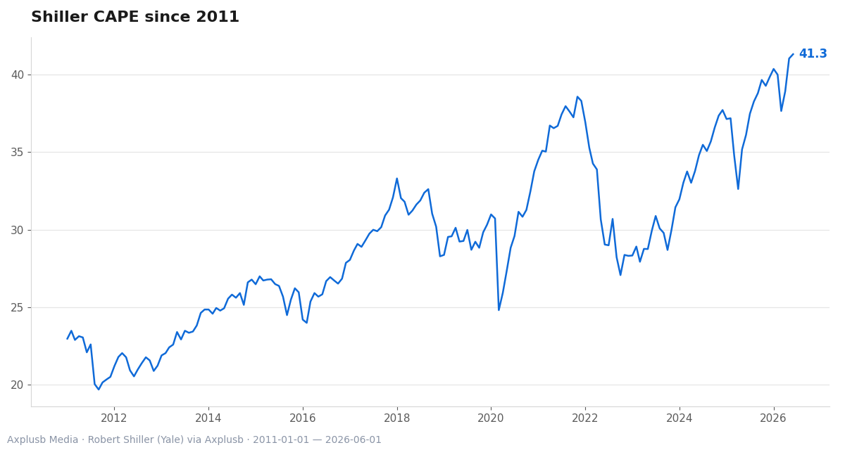
Late‑cycle conditions concentrate uncertainty. The LTCMA lens highlights resilience at the portfolio level, not just tactical bets, because drawdowns late in the cycle carry larger opportunity costs. That view treats tail protection as a strategic question about funding, governance, and re‑risking capacity.
The macro layer adds more pressure. Fat‑tailed shocks can propagate through trade, funding, and policy channels in uneven ways, which raises the value of risk sharing for investors and countries alike BIS Working Paper No. 958.
Institutional desks also stress the portfolio interaction term. Goldman Sachs argues the main value of tail hedges appears when they allow a higher core risk budget with tolerable downside, not as standalone alpha sources in quiet times. That logic reframes hedges as enablers of strategic equity exposure within a controlled loss budget.
For investors living with political and policy shocks, this is not abstract. We have shown how to build processes that face event risk without flinching in Assessing Portfolio Risk in an Era of Geopolitical Uncertainty.
Common misconceptions and simple myths busted
Myth one: “Options are free insurance.” Buying out‑of‑the‑money puts has had a negative average return across long samples. AQR documents that this drag is persistent, while multi‑asset trend strategies posted positive long‑run returns AQR tail‑risk white paper.
Myth two: “One hedge fits all.” Option overlays, trend‑following, and de‑risking solve different problems. A single structure cannot offer precise floors, cheap carry, and broad crash protection at once. Institutions mix layers because the trade‑offs are real and context‑specific.
Myth three: “Volatility equals tail risk.” Vol spikes are common and often mean‑reverting. Tail risk refers to the extreme left side of the outcome distribution, which can occur with or without high realized volatility. The LTCMA framework makes this exact distinction in its risk taxonomy.
Myth four: “Timing solves cost.” Industry simulations around the 2020 selloff show that option hedges helped only if entered at the right time. Outside those windows, simple allocation changes, such as lowering equity weight, often matched or beat option overlays.
How to measure what you’re insuring: VaR, Expected Shortfall and simulation practicalities
You cannot manage what you do not measure. Value at Risk is intuitive but blind to losses beyond the chosen quantile. Expected Shortfall, also called Conditional VaR, averages losses in the tail and is a coherent risk measure for stress scenarios according to the Federal Reserve’s methodological work Federal Reserve FEDS paper.
Complex portfolios rarely yield closed‑form tail metrics. The same paper details nested simulation, where outer scenarios drive market states and inner loops reprice positions. It also discusses bias problems and tools such as jackknife estimates to trim bias when compute budgets are tight Federal Reserve FEDS paper.
AQR evaluates tail hedges using CVaR because hedges should target loss severity, not just frequency. Align sizing to the loss you promise to absorb, and keep the metric stable across regimes AQR tail‑risk white paper.
This is a quant job, but the objective is plain. Define what you fear, measure it with CVaR, and size the hedge to the shock that matters.
The toolset: direct option hedges, indirect hedges and portfolio design
Direct hedges buy convexity. Out‑of‑the‑money puts and put spreads can draw a line in the sand on losses, with known premiums. AQR shows that this precision has carried a negative average return across time AQR tail‑risk white paper.
Indirect hedges diversify the path. Multi‑asset trend‑following tends to pick up sustained down moves and posted positive long‑run returns in the same study. De‑risking the core allocation cuts drawdown at the source, which the LTCMA notes can rival overlays when insurance is rich.
Industry tests around 2020 reach a clear message on cost. Buying deep puts or collars was expensive on average, and allocation changes often matched their payoff except under perfect timing. That is not an argument against options, it is a warning about budgets and cadence.
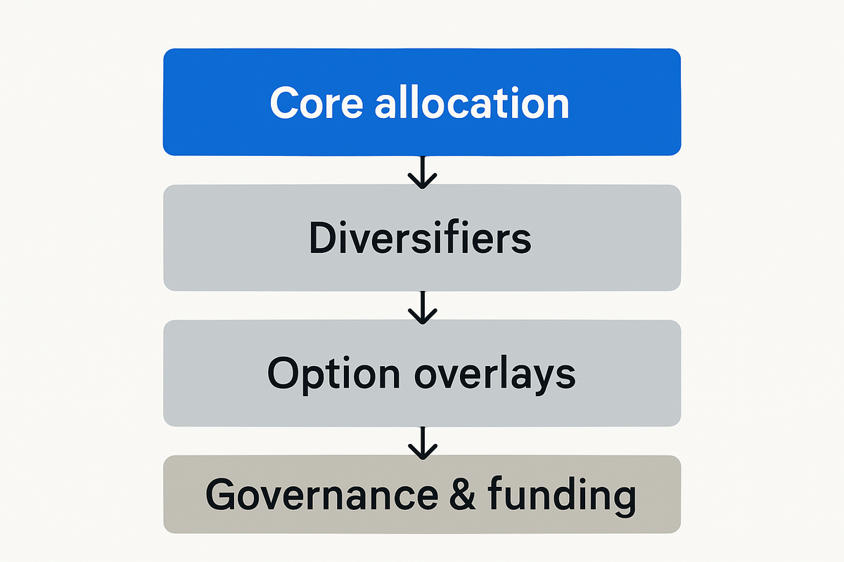
Practitioners often combine layers. A robust core, diversifiers that can run in stress, and tactical option use for known events form a workable stack in real governance settings.
| Hedge type | What it targets | Carry profile | When it shines | Key caveat |
|---|---|---|---|---|
| OTM puts / collars | Precise loss floors | Negative on average | Fast crashes, gap risk | Premium drag outside stress |
| Trend-following (multi-asset) | Sustained downtrends | Positive over long run | Prolonged selloffs | Can lag sharp rebounds |
| De-risking (lower equity) | Smaller drawdowns | Neutral | All regimes with high valuations | Opportunity cost in bull runs |
| Diversifiers (rates, macro) | Non-correlated returns | Mixed | Policy shocks, growth scares | Correlations can change |
Check how disciplined your portfolio really is.
Cost, value and sizing frameworks: from standalone alpha to enabling risk taking
The debate is not whether hedges “make money” in quiet times. Goldman Sachs frames the true value as enabling a higher strategic equity weight while keeping downside inside a defined CVaR. The standalone return of the hedge may be small, yet the portfolio‑level gain can be large when the core is bigger.
This leads to budgets and “reliability” metrics. A reliable hedge pays when the portfolio needs it most and does not erode carry beyond plan. That framing helps boards accept a steady premium for insurance that unlocks a superior long‑run mix.
AQR’s evidence fits this approach. Trend hedges have shown better long‑run cost efficiency than always‑on put buying, which informs how you allocate the hedge budget across tools AQR tail‑risk white paper.
The LTCMA’s distinction between volatility management and tail protection also matters here. If the goal is a tighter drawdown bound, accept explicit costs and plan funding, rather than hoping standard risk models will cover the left tail.
Historical evidence and stylised simulations: what backtests tell us
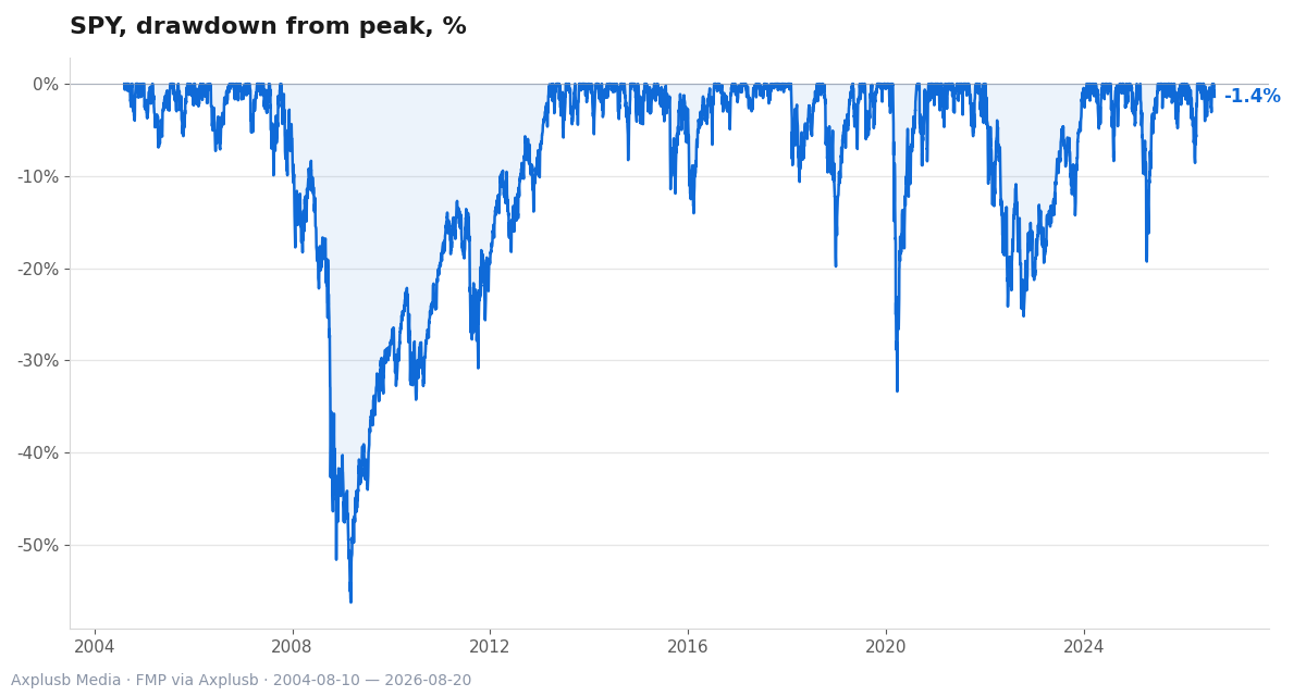
Backtests are not oracles, but they focus the mind. AQR’s long history comparison finds option buys carry a persistent premium, while trend‑following delivered positive long‑term returns and material crisis gains AQR tail‑risk white paper.
MSCI’s simulations around 2020 offer a clean counterpoint on practicality. Option‑based hedges helped during the drawdown but were costly outside it, and simple allocation moves often matched them in long samples unless timing was perfect.
Goldman Sachs adds a different lens. They show that portfolios can run higher equity beta when a reliable hedge sits behind them, which compounds value over long horizons. That shifts the question from “did the hedge beat cash” to “did the strategy improve the whole system.”
If you want a deeper dive on drawdowns and sequencing risk, see our piece on Advanced Techniques for Managing Portfolio Drawdowns in Volatile Markets.
Counterarguments and limitations: timing risk, model risk and opportunity cost
First, timing risk is real. Industry evidence shows that many option programs only look good when measured around the crash window, and they lag outside it. A plan that depends on perfect entry points will fail most investment committees.
Second, model risk sits inside your CVaR. The Federal Reserve’s work shows that ES estimation can be biased in complex books and needs careful simulation design and bias correction Federal Reserve FEDS paper.
Third, the premium on long volatility is persistent. AQR shows a negative average return for put buying across regimes, which is the cost side of insurance AQR tail‑risk white paper.
Finally, behavior can undo good math. Frequent repositioning adds slippage and governance friction. That is why process, pre‑set triggers, and clear funding rules matter as much as the instrument choice.
A practical playbook: layers, diagnostics and next steps
Start with objectives. Define the maximum loss you will accept over a horizon, then express it as a portfolio CVaR. Align stakeholders on what the hedge should do and when it is allowed to cost.
Choose your layers. Use a robust core allocation, add diversifiers that can work in stress, and reserve options for events or regimes where precision matters. Treat put buying as a budgeted tool, not a belief system.
Size and test. Apply a reliability mindset from the Goldman framework when picking instruments and budgets. For complex exposures, build nested simulations, monitor ES bias, and use jackknife or related adjustments where compute is scarce Federal Reserve FEDS paper.
Monitor and govern. Decide in advance how you will roll, when you will re‑risk, and how gains from hedges fund future risk. Keep the metric stack stable across regimes so you can compare like with like.
- Set a CVaR target the board can live with.
- Allocate across layers: core design, diversifiers, and tactical options.
- Budget hedge carry and define reliability thresholds.
- Build nested simulations and track ES estimation error.
- Pre‑commit roll rules and re‑risk triggers.
- Review outcomes after stress and recycle gains to core risk.
Stress test your plan before the market does. For the human side of sticking with it, see The Role of Investor Psychology in Volatile Markets: Strategies for Resilience and The Psychology of Bear Markets: Navigating Investor Behavior in Tough Times.
Related reading
- Advanced Techniques for Managing Portfolio Drawdowns in Volatile Markets
- The Role of Investor Psychology in Volatile Markets: Strategies for Resilience
- The Psychology of Bear Markets: Navigating Investor Behavior in Tough Times
- Assessing Portfolio Risk in an Era of Geopolitical Uncertainty